So, you’ve created a table for your expenses (click here to see how to create one) but how do you format it to accept currency, dates and any other data you want to include in it?
Below are simple step by step instructions to show you how. I must apologise in advance for the length of this post, but it does show instructions one at a time (you can enlarge the images by double clicking on them).
Don’t forget, if you don’t have time to read it all, you can always press the printer icon at the end of the post to print / save it to a PDF file. 🙂
DATE
Type in the date of the first entry that you want to make. Highlight that cell and the rest of the column. There are several ways of formatting a cell.
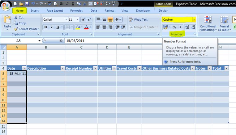
1. Make sure you’re in the Home tab, and go the Number section in the ribbon at the top of the page.
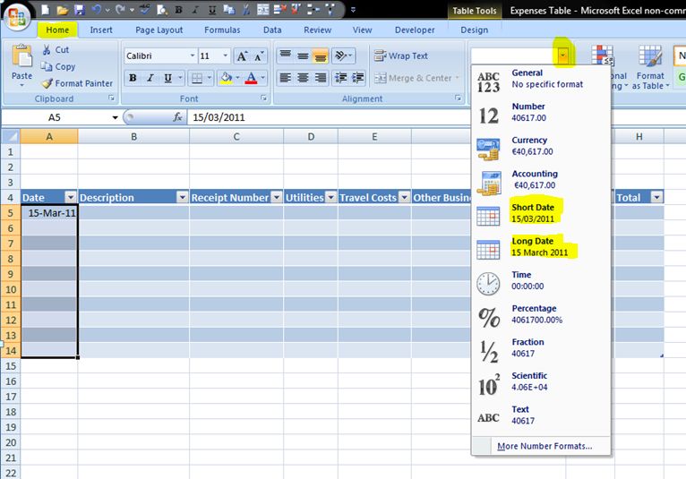
Click on the drop down arrow and it will list shortcuts to the most popular formats. Click on either the Short Date or Long Date and the highlighted column will change.
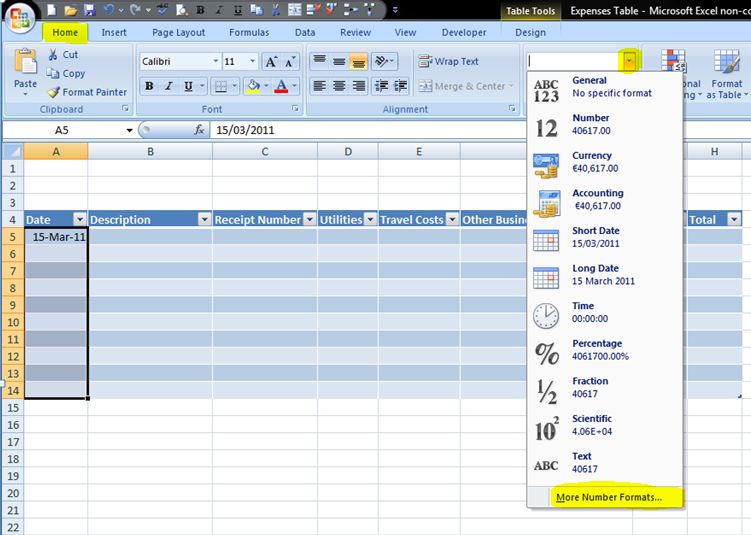
2. If you prefer not to use either of these options, then click on More Number Formats… at the bottom of the list.
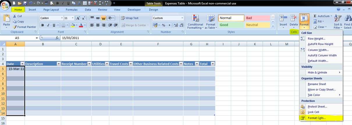
3. You could also go to the Cells section in the Home tab, click Format then Format Cells… – this will bring up the same table as clicking More Number Formats (in step 2).
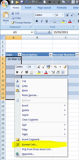
4. Or you could right-click your mouse over the highlighted cells, and go to Format Cells… this will also bring up the same table as the previous 2 ways.
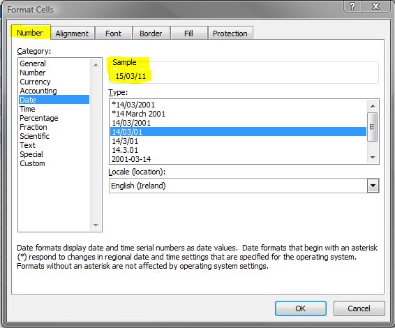
Whichever way you choose, an extensive menu will be displayed for formatting cells. The Date is already selected as it recognises that you already have a date format in the highlighted cells. You can choose whichever you prefer from this list. A preview of it is shown in the Sample box.
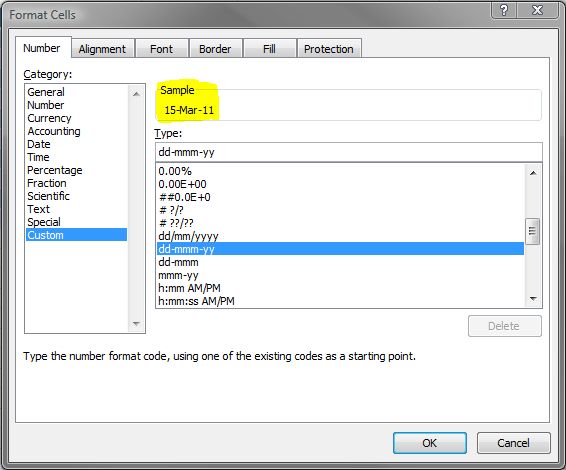
If you still prefer a different format to these, then you can choose a custom one. Select the Custom category on the left side and it will show a selection of other formats on the right. Again, whenever one is selected a preview is shown in the Sample section
*Quick key – dd=day (2 digits) / mm=month (2 digits) / mmm=month (3 letters) / yyyy=year (4 digits) / yy=year (2 digits).
The one I always tend to go for is dd-mmm-yy. Click OK once you’ve chosen and the date column will now be formatted the way you like.
DESCRIPTION
This will tend to be text as it will be the name of a company / supplier – no formatting will be needed for this.
RECEIPT NUMBER
This is up to you how you number your receipts (or if you even have a column for this) – I tend to go for simple 1, 2, 3 etc – again no formatting is needed.
EXPENSES HEADINGS
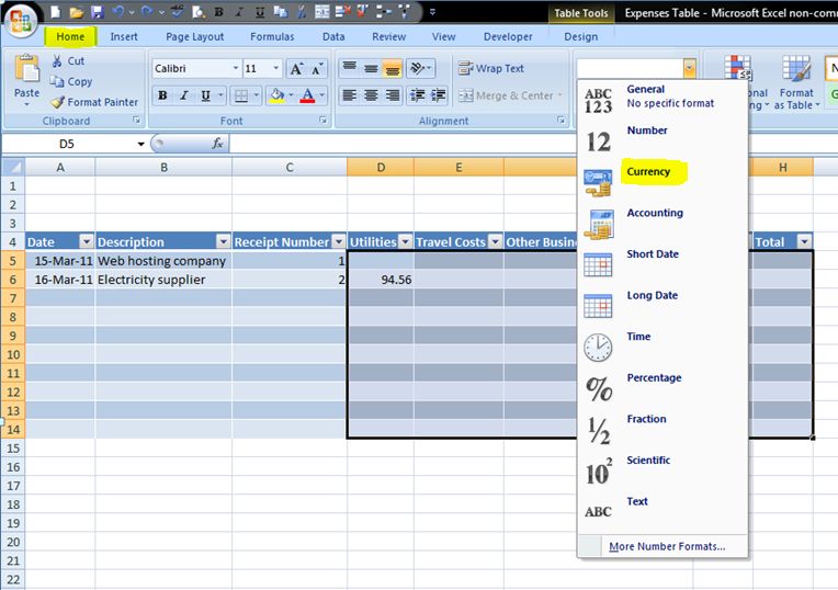
Enter the cost of the first expense. You’ll notice how it just lists it as an ordinary number, if you want to change this to show currency then there are several ways to do this. Highlight the cells you want to include in the formatting.
1. Making sure you’re in the Home tab, go to the Number section on the ribbon, click the drop down arrow and select Currency.
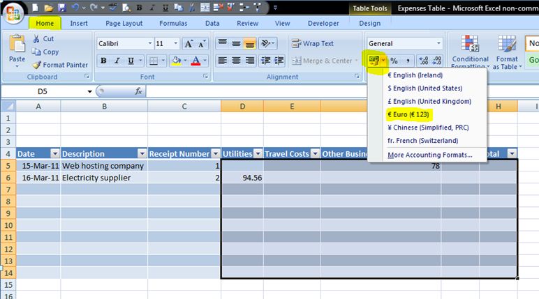
2. You could also click on the drop down arrow to the right of the shortcut icon for currency (in the Number section on the ribbon), you can then choose the currency type e.g. Euro, Sterling etc.
This will also automatically put your decimal places to 2. If you want to change the number of decimal places, then select the icons within the number section on the ribbon (hover over them & it will tell you what they do).
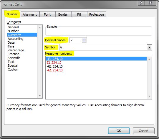
3. You could also click on drop down arrow in the Number section and go to More Number Formats… on the list (or right-click mouse and select Format Cells…), and it will bring up the table below. Currency is already selected – here you can choose the number of decimal places, the symbol for the currency type, and whether you want any minus values to be shown in red.
ALIGNMENT
The last thing to format is the alignment of the text within the cells. It looks fine the way it is at the moment, but you may prefer some of the text to be centred, for example the Date and Receipt Number columns.
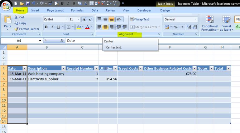
Highlight the column you want to format (e.g. date), make sure you’re in the Home tab, go to the Alignment section on the ribbon and select centre (again hover over the icons for description). Repeat for other columns as necessary.
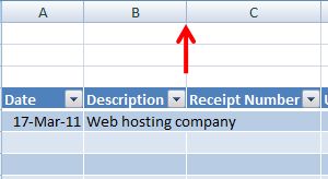
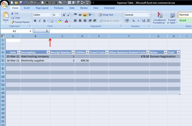
You may notice that some of your text that you’ve entered overlaps into the next column as its too long. To re-size a single column so it automatically fits the text, hover on the dividing line between the column headers to the right of the column you want to change (for example B and C).
Wait for the cursor to change to the shape pictured below, then double click and the column width will automatically re-size to fit the text.
You can do the same for individual rows, by hovering on the bottom dividing line between row numbers and double clicking – the row height will automatically re-size to fit text.
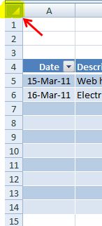
To save time, if you want to re-size the whole worksheet (rows and columns), then click on the square in the top left corner (between A and 1), this will highlight the whole worksheet.
Double click on a line between any of the column headers (e.g. B and C), this will re-size all column widths. Double click on a line between any of the row numbers (e.g. 3 and 4) and this will re-size all row heights.
You may have noticed that a couple of the columns are alot wider than the rest in order to fit the text in (for example Other Business Related Costs), we can make this column narrower by wrapping the text.
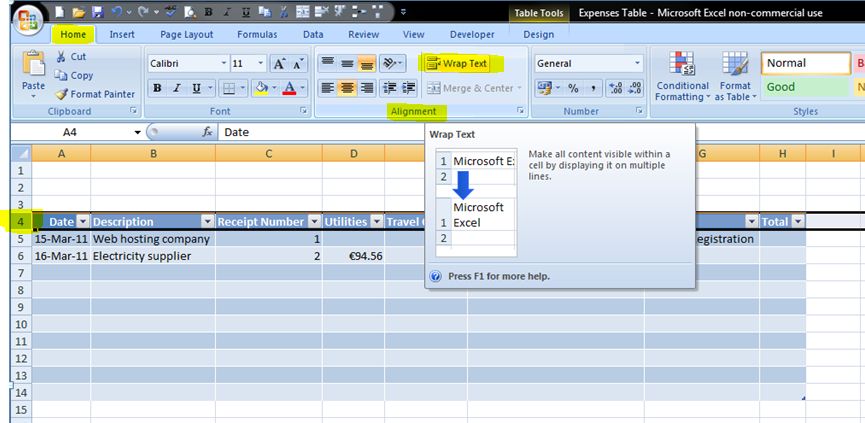
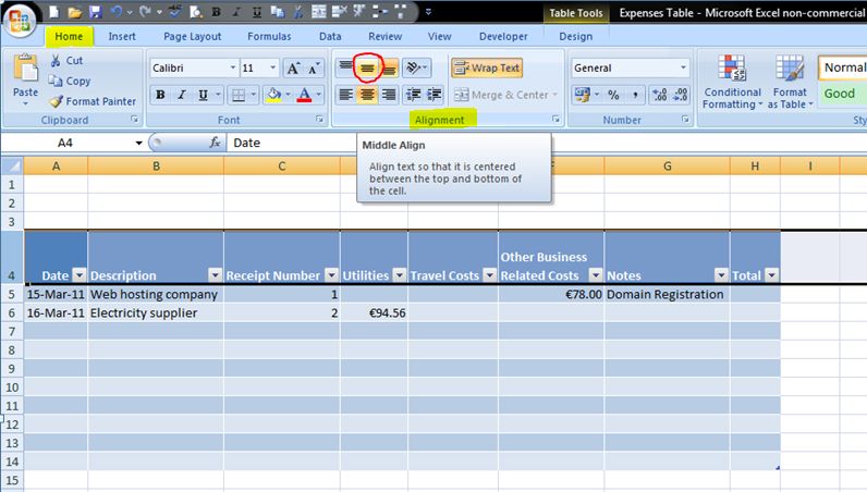
Highlight the whole row containing the table headers by clicking once on the row number (in this case 4). Make sure you’re in the Home tab and go to the Alignment section on the ribbon. Click on the Wrap Text button.
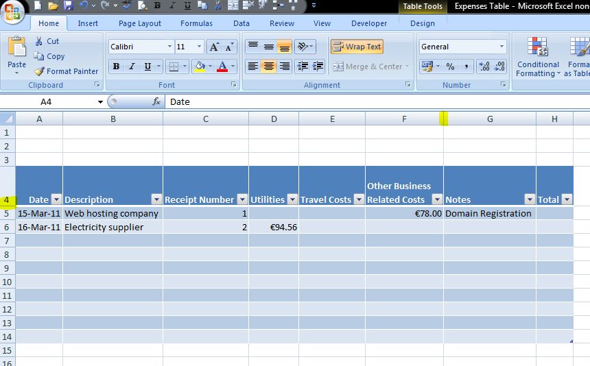
It doesn’t look like anything has happened, but if you increase the row height (by dragging the line down under the row number), and shorten the column width (by dragging the line to the right of the column), you will notice how the text has now wrapped itself into multiple lines within the one cell.
You can then centre these headings if you wish by selecting Middle Align (making sure the row is highlighted).
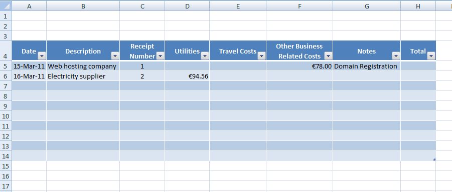
Again, highlight the whole worksheet, double click a line between column letters and a line between row numbers to have everything autofit. So the table ends up looking a bit like this:
If you’re still reading this then I must congratulate you for making it to the end of what must be my longest post EVER! 🙂
I hope you’ve found these guidelines useful. I’ll be posting more about this table in the coming weeks, including how to include formulas and how to set up the page ready to print.

