Don’t you just hate it when column headings in a table in Excel disappear when you scroll down?  How are you supposed to remember which information goes in which column of the table?  Well, you can freeze the row so its always visible.

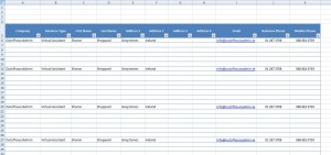
Below is an example of a table that you might use to input all those business cards you collect from networking.  (Don’t forget if you want to enlarge the images, just click on them).

(NB if you have stacks of business cards but don’t have time to collate the information, outsource it to a Virtual Assistant…… its what we’re here for ;))

If you need help inserting a table to start with, click here for my previous tutorial.

You’ll notice as you scroll down that the whole table moves down.  This is no good if your table is hundreds of rows long, so how do you get the headings to always show at the top of the page?

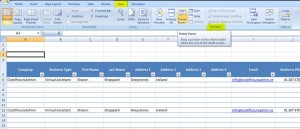
Firstly, go to View in the ribbon and click on Freeze Panes (in the Window section)

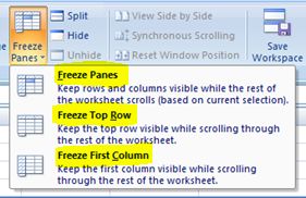
This will then bring up the following menu:-

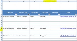
Freeze Panes – This freezes the rows above and columns to the left of the cell you’ve selected.  For example, if I click on cell E13 in the table and select Freeze Panes, you’ll notice a line has appeared between columns D and E, and between rows 12 and 13.

When you scroll down, all rows above 13 are still showing…. scroll right and all columns to the left of column E are still visible.  Below is an example showing how columns have jumped from D – H, and rows have jumped from 12 – 34 after scrolling.

To undo the frozen panes at any time, just click back on Freeze Panes (on the View tab in the ribbon), and you’ll see there is now an option to Unfreeze Panes.  Click this and it all returns to normal.

Freeze Top Row / Freeze First Column – These 2 options do exactly what they say.  Click on Freeze Top Row, and it freezes the very first row of the spreadsheet, no matter what cell you’re currently in.  Click on Freeze First Column, and again it freezes the very first column which is visible on the spreadsheet (usually column A, unless that column is hidden).

Neither of these 2 options are any good for our table as it would still mean the column headings would move when we scroll down.

I want to be able to see the column headings when I scroll down, and the Company Name if I scroll over to the right, so click on cell B6, and select Freeze Panes.

Now scroll down and right to see if its worked….. and that’s how to freeze rows / columns in Excel 2007 🙂

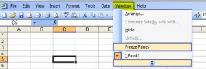
To do the same in Excel 2003, you need to click on Window, and select Freeze Panes.

This does exactly the same as the Freeze Panes option in 2007, unfortunately you don’t have the choice of freezing the top row or first column in 2003.

If you have any questions with any of the above, please feel free to leave them in the comments section below 🙂