If you have a lot of data in a spreadsheet and you only want to focus on a certain area, it’s sometimes useful to hide the columns and/or rows that you don’t want to see.  There are 3 different ways of doing this, all of them quick and easy 🙂

To hide columns…..

1) The Ribbon Way

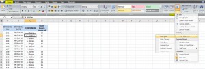
Click on a cell in the column that you want to hide. Make sure you’re on the Home tab in the Ribbon – go to the Cells section – click on Format and choose Hide & Unhide – Hide Column.

2) The Mouse Way

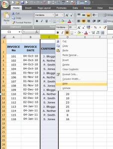
Select the whole column by clicking on the column header (A, B, C etc) of the column you want to hide – right click – select Hide.

3) The Keyboard Way

Select a cell in the column you want to hide – press Ctrl+0.

To hide rows…..

1) The Ribbon Way

As before, click on a cell in the row that you want to hide. Make sure you’re on the Home tab in the Ribbon – go to the Cells section – click on Format and choose Hide & Unhide – Hide Row.

2) The Mouse Way

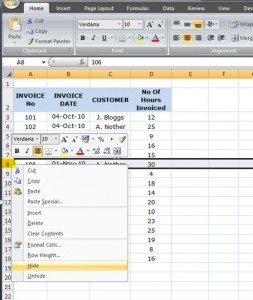
Select the whole row by clicking on the row header (1, 2, 3 etc) of the row you want to hide – right click – select Hide.

3) The Keyboard Way

Select a cell in the row you want to hide – press Ctrl+9.

The same methods go for unhiding columns/rows:

To unhide a column – select a range of cells to the left and right of the hidden column, choose any of the methods above but select unhide instead of hide.  With the keyboard shortcut press Ctrl+Shift+0 to unhide.

To unhide a row – select a range of cells above and below the hidden row, and again select unhide when using the above methods, or Ctrl+Shift+9 if using the keyboard shortcut.