The VLookup formula is my favourite function of Excel; I use it all the time and it saves me so much time!  The formula looks up data from one worksheet and uses it in another. Below is an example of how I would use it with a product inventory.

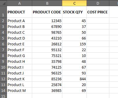
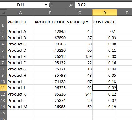
Let’s say we have exported product stock information from another source into an Excel spreadsheet. This worksheet contains the product name, product code, and stock levels.

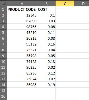
We also have another separate spreadsheet saved on the pc which contains the product code and cost price for all of the products.

We want to insert the cost price into the stock levels sheet so we can work out total costs of what we have in stock.  We have to find the common data found in both sheets in order for the Vlookup formula to work.  In this case it would be the Product Code…

With the Vlookup formula we’re asking it to look up the product code in the cost spreadsheet and insert the relevant cost price into the stock spreadsheet.

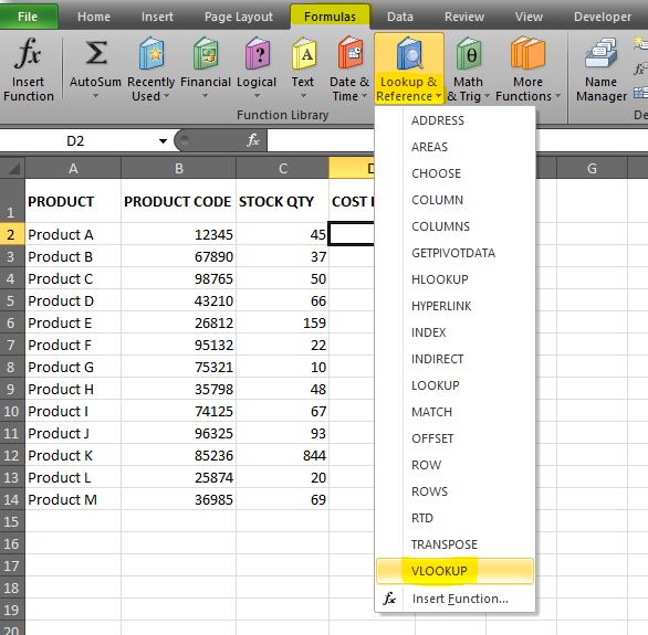
In the stock spreadsheet click on the first cell where we want to insert the formula (e.g. cell D2), click on the Formulas tab on the ribbon, click the drop down arrow next to Lookup & Reference, and select VLOOKUP…

This will open the Functions Argument dialog box…

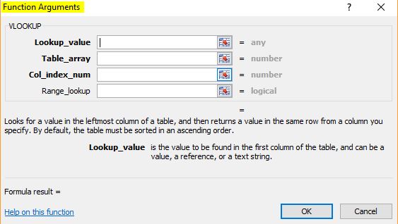
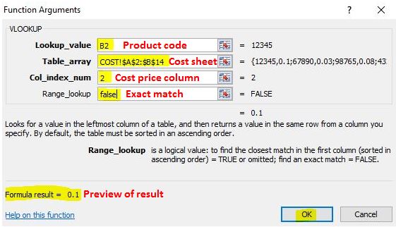
The Vlookup is split into 4 parts:

Lookup_value:  This is the starting point of the formula. This is the cell that contains the data we want to look up. In this example that would be cell B2 (Product Code).

Table_array:  This is the range where data is retrieved from, so in this example it would be the sheet containing cost prices. Ranges can be in the existing worksheet or a different one.

Col_index_num:  This is the number of the column in the table array that has the information we need. The first column of values in the table is 1. In our example it would the Column B containing the cost prices, so that would be column number 2.

Range_lookup:  This field defines how close the information has to match e.g. do we want the information to match exactly or just be as close to it as possible.

The image below shows the dialog box filled in. It also gives us a preview of the result so we know if we’ve included the right information.  Once filled in click OK…

There are some rules to remember with the table array in order for the Vlookup formula to work…

RULES TO REMEMBER…

• The LEFT column must contain the data being referenced. So in our Cost sheet the Product Code must be on the left.
• Values in the leftmost column of the lookup range must be unique, i.e. no duplicates. In our example the Product Code can only appear once in the table array.
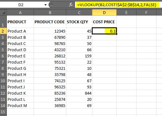
• If the formula is to be copied anywhere else the table array referenced in the formula needs to be an absolute reference. In other words, the table array needs to stay fixed and not move down a row if you copy the formula down.  To make sure the table array is absolute, press F4 to insert a $ before the column & row figures. For example in the image above you’ll see under Table_array $A$2:$B$14; this means the array will stay within cells A2 to B14 no matter where we copy the formula to.

The cost price has now been inserted into cell D2…

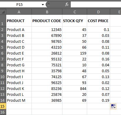
Double click the fill handle in the bottom right corner of the cell and the formula will automatically copy down to the end of the list…

We can always spot check values in the table array on the other sheet to double check it’s brought through the correct figures.

Remember that Column D still contains the Vlookup formula. If we want to remove the formula & only keep the values then we need to paste special as values.

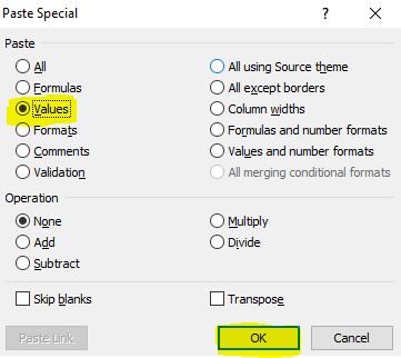
Select Column D and press Copy (or Ctr+c), right click the column and choose Paste special…

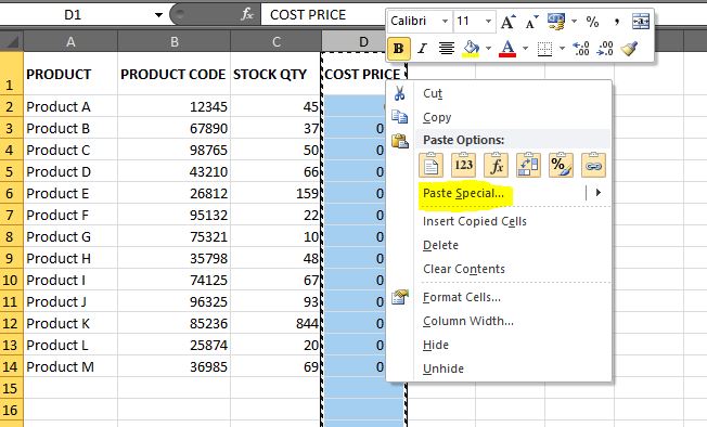
This will open the paste special dialog box where you can choose how you want to paste the cells. You want to get rid of the formulas and only keep the actual value of the cell, so click on Values and press OK.

Column D now only contains the actual cost prices…

And that’s it! I use Vlookup all the time and I find it especially useful when combining 2 different sheets into one. I hope you do too 🙂