I use conditional formatting in a lot of my spreadsheets, mainly to show me when dates are coming up, e.g. when a training date is less than a week away, or if an invoice is overdue etc.  Most of the time I use it to format individual cells (see my earlier tutorial on how to do this), however a client recently asked me how to highlight the entire row that contains that cell. This tutorial shows you how 🙂

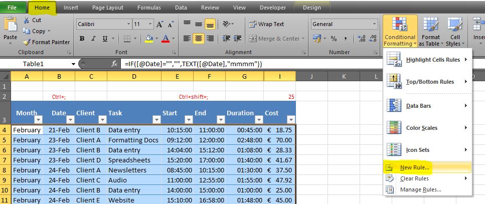
In the example below we want to highlight the entire row where the cost (column I) is less than €25.00…

We first select the entire range of data we want to format, excluding the column headings (in this example A4:I16)…

Go to the Home tab on the ribbon, click Conditional Formatting, then click New Rule…

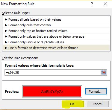
The New Formatting Rule dialogue box appears.  In the Select a Rule Type section, choose Use a formula to determine which cells to format…

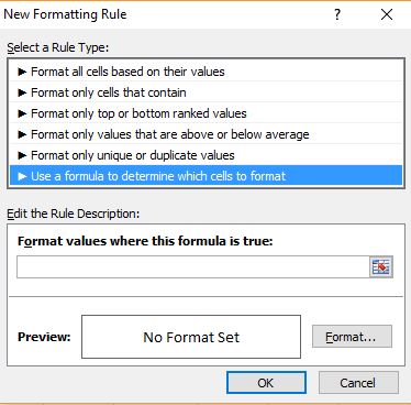
In the Format values where this formula is true field, we need to create a formula that evaluates to either TRUE or FALSE. For cells where this formula evaluates to TRUE, conditional formatting will be applied.

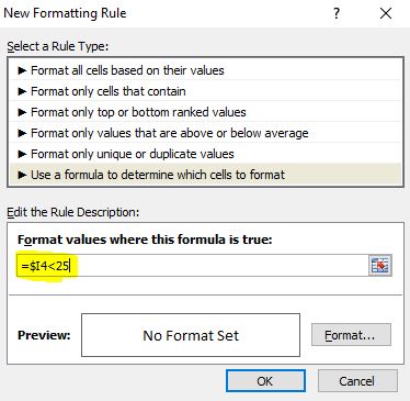
We want to highlight the rows where the value in column I is lower than 25, therefore we need to type in the formula =$I4<25. We want to ensure that the conditional formatting for all cells in the selection refers to column I, so we use absolute ($) column references.

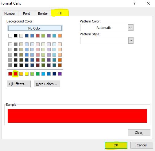
We then need to choose the formatting to apply to rows where this formula is TRUE. Click Format… then click the Fill tab, choose a background colour and click OK. In this example I’ve chosen red…

We can then see a preview of the cell formatting…

Click OK and we’ll now see entire rows filled in red where the cost in column I is less than 25…

That’s it! I hope you’ve found it helpful 🙂