Once you’ve created your pivot table and got to grips with the data that you want to include, you might want to format it.  Listed below are the steps needed to format your table:-

To format the style of the pivot table…

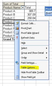
If you want to change the layout of the table, click on the drop down arrow besides the Pivot Table button, and select Table Options…

This opens up a dialogue box where you can pick and choose which options you want available for your pivot table, e.g. whether you want to show grand totals etc, you can also change the name of your pivot table in this window…

Another easy way of bringing up the same dialogue box is to right click your mouse anywhere on the pivot table and choose Table Options…

To format the values within the pivot table…

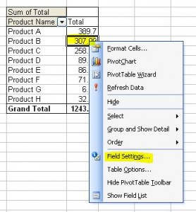
If you want to change the format of the actual data, e.g. you want the totals to have € symbol, you need to go into the Field Settings option.  Firstly click on a cell in the column of where you want to format e.g. any of the total figures in the pivot table, then click on the Field Settings icon in the Pivot Table toolbar…

Again, another way to access this is to right click your mouse on any of the total figures in the pivot table and choose Field Settings…

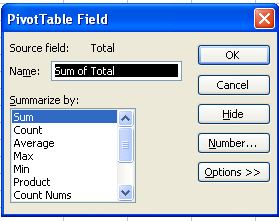
Whichever way you do it, the Field Settings dialogue box will open and you can choose the function of the column e.g. sum, count etc.

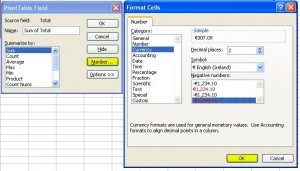
Click on Number… and you can format the cells to apply the currency format etc…

Click OK to close each dialogue box and you’ll see that the pivot table has now been formatted to your specifications…

And that’s it – again it’s just a matter of having a play around with the different formats until you find one that suits your purpose.

I hope you’ve found this series of tutorials helpful, and if you have any questions, just leave them in the comment section below 🙂