Whenever we have a large list of values (whether it’s numbers or text), there is always a risk of duplication.  An earlier post shows you how to hide or remove these duplicate values, but what if you actually want to keep them but just have them highlighted?  That’s where conditional formatting comes in…

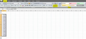
The example below shows just a random list of numbers.  The first thing to do is highlight the section you want to check, and click on Conditional Formatting which is in the Styles section in the Home tab of the ribbon…

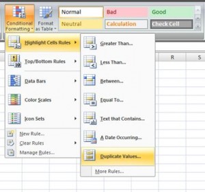
Next click on Highlights Cells Rules, and choose Duplicate Values…

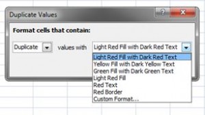
A dialogue box will open where you can then choose how your cells will be highlighted…

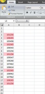
Click OK, and you’ll see that all cells containing duplicate values are now highlighted…

And that’s it! A quick and easy way to identify duplicate values.  The formatting will remain in the cells you have chosen, so as soon as you change any of the duplicated values the formatting will automatically update 🙂