Once you have a pivot table created (click here for my tutorial on how to create one), you will need to know how to keep it updated with any new data that you add or change.
1. Update pivot table with amended data
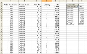
Below is the pivot table we created last time…
Let’s say a mistake was made when entering the data in the original table, and we now need to change some of the quantities. We can change that on the data table but the pivot table also needs to reflect these changes.
You’ll see the top 5 rows of the data table now have quantities of 10 therefore the totals will have changed…
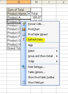
In order to update the pivot table, all we need to do is right click anywhere in the pivot table and click Refresh Data…
And that’s it 🙂 The pivot table updates itself with the new totals from the data table.
Below is how to update the table if we add new rows to the data table.
2. Update pivot table to include extended range of data
If we add more rows of data to the table, you’ll see that the pivot table remains the same…
This is because the data range, that was set up at the very beginning of the creation process, still goes from cell A2 to cell E27. Our data now goes beyond this range so we need to change it.
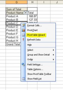
The quickest way to do this is to right click anywhere on the pivot table and select Pivot Table Wizard…
This will open up the wizard that we used in creating the pivot table originally, click < Back…
And it takes us back to Step 2 of the wizard which was selecting the range of the data we want to use. All we need to do is change the range to include the new rows, so it will go from cell A2 to cell E34. Then click Finish…
You’ll see that the pivot table’s total has now changed to include the whole range.
And that’s it!
Next week I’ll show you how to format your pivot table 🙂


