A few weeks ago I asked followers of my Facebook page if they wanted me to cover a specific topic in a tutorial, the majority of the replies I received were for pivot tables. It seems a lot of people want to use them but are just not sure where to begin, so in the words of Aladdin’s genie “your wish is my command”! 🙂
Firstly, for those of you who don’t know what a pivot table is, it’s a fantastic tool in Excel that sorts and summarises data, and then inputs it into another table which is a bit more user friendly, more readable. For example, if you have data that shows details of every customer that has bought your product over the last 5 years, by using a pivot table you can find out which product is most popular, which town/county/country most of your customers came from, and whether your customers were male or female etc, depending on the data you have available.
Below is a short tutorial on how to set up a very simple pivot table in Excel 2003.
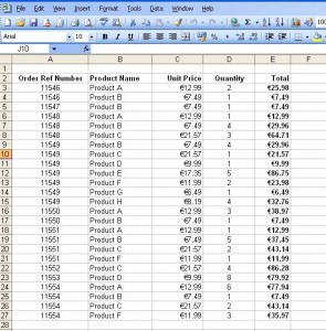
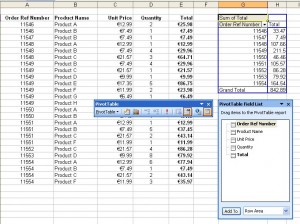
In Sheet 1 is a list of data that we’ll use for the pivot table, it basically just lists a reference number, product name, unit price, quantity and a total…
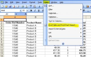
Click on Data on the toolbar, and select PivotTable and PivotChart Report…
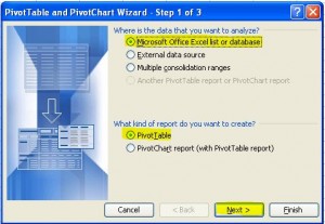
This will automatically open up the pivot table wizard, and it’s just a matter of following the step by step instructions. Make sure that the “Microsoft Excel list or database” and “PivotTable” options are chosen, then click Next…
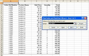
Select the range of data that you want to use for the pivot table, in this example it has automatically highlighted the range A2:E27, then click Next…
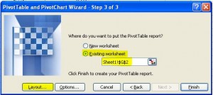
It then asks where you want the pivot table to appear, either in a new worksheet or in the existing one. For this example we’ll choose existing worksheet, click on an empty cell where you want the pivot table to appear (in this example cell G2), then click on Layout…
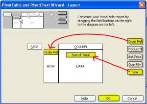
You can now construct your pivot table by dragging the fields that you want to appear in the Page, Row, Column, and Data sections of the pivot table. For this example, we’ll drag the Order Ref Number field to the Row section and the Total to the Data section, then click OK…
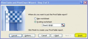
Click Finish, and the pivot table should appear in cell G2 next to the existing data…
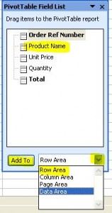
You’ll notice that there is also another toolbar that has appeared next to the pivot table – this is a shortcut toolbar so you can make changes to the pivot table as and when you want to. For example, you might want to see the product name instead of the reference number, so all you need to do is highlight Product Name, choose which area you want to add it to (for example Row) and click Add To…
Don’t panic if you don’t see the above menu, just click anywhere on the pivot table and it should appear (if it doesn’t, go to View on the toolbar, click Toolbars, and make sure Pivot Table is ticked) 🙂
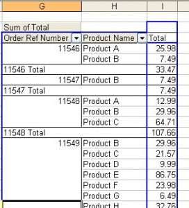
The pivot table will now look something like the image below, showing the Reference Numbers, Product Name and Total…
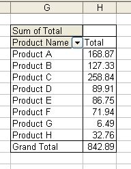
To remove the reference numbers, just click on the cell which contains the Order Ref Number title (shaded grey), and drag it into the Field List box (where you highlighted Product Name in the above step), the cursor will change to include a red cross, release the mouse and the pivot table will change to show just the Product Names and Totals as below…
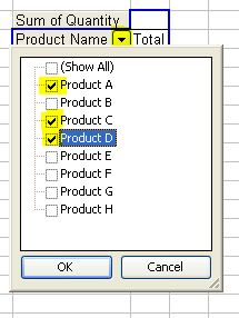
The table automatically applies a filter so you can choose which data you want to see, for example you may only want to see Product Names A, C and D, just click on the drop down arrow next to the title and tick the boxes of ones you want to see…
Obviously this tutorial is just showing you the basics, a lot of creating a pivot table is trial & error and it’s just a matter of working out the best way of organising the data you want to see. There are other options within it to allow different formats of fields, different views etc. Pivot tables are so flexible so once you have the basic one set up, just have a play around with the data. The next tutorial will show you how to format your table and what to do if the original data changes.
I hope you find this useful, but if you have any questions about this tutorial, please leave them in the comment section below 🙂

