
One of my missions as a Virtual Assistant is to try to save clients time. I was with a client the other day and noticed they had downloaded information from their accounting software into Excel. They were retyping data that was already there just because they wanted the information in separate columns. I showed them a quick and easy way of doing this by using formulas. Below is an example of how to do this 🙂
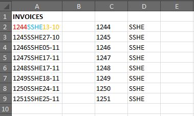
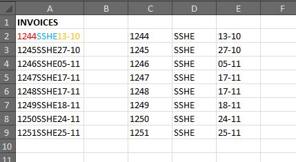
Let’s say we have a list of invoices downloaded into Excel, each cell contains the invoice number (4 digits), the customer code (also 4 digits) and the due date (5 characters including the “-“)…
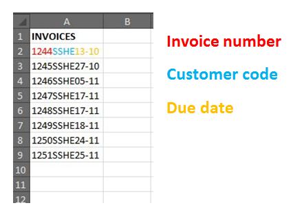
In order to have these 3 elements in separate columns, we need to use the Left, Mid and Right functions.
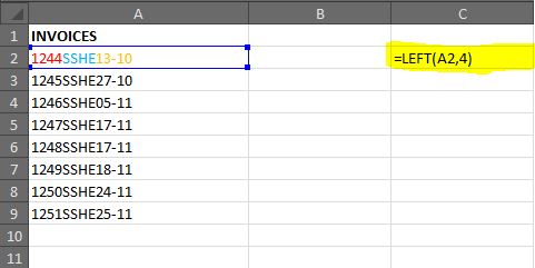
Firstly click on the cell where you want the first section of data to appear. In this example we want column C to contain the invoice numbers, column D to have the customer codes and column E to contain the due dates.
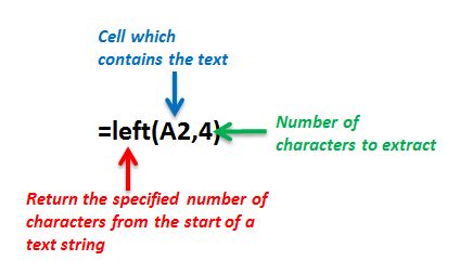
So, in cell C2 we need to type in the following formula:-
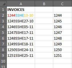
This formula is then copied down to the end of the list, so column C contains the invoice numbers…
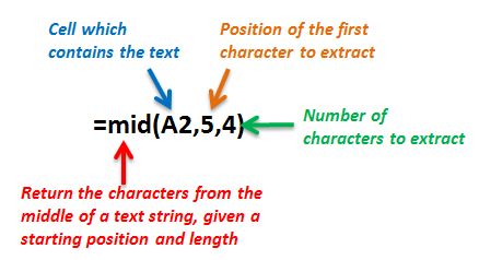
Next we want to do the same for the customer code, but this isn’t at the start of the text, this is in the middle of the text – for this we use the Mid formula. Click on cell D2 and type the following…

This formula is then copied down to the end of the list, so column D contains the customer codes…
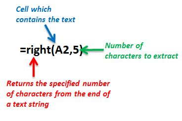
Next we want to do the same for the due date, again this isn’t at the start or middle of the text, this is at the end of the text, and for this we use the Right formula. Click on cell E2 and type the following…
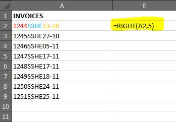
Again, the formula is then copied down to the end of the list, so column E contains the due dates…
And that’s it – 3 quick and easy formulas to help you save a bit of time 🙂