
This is the first part of a series of tutorials to show you how easy it is to create a working timesheet in Excel. This tutorial will show you how to:
a) Set up the spreadsheet with relevant column headings and different sheets
b) Format the data into a table
c) Create the necessary lists to be used in the data validation
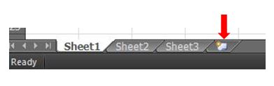
So, to begin open up a new blank workbook in Excel and make sure there are 3 sheet tabs showing at the bottom of the page. If you don’t see 3 tabs visible, press Shift+F11 to insert a new sheet or click on the icon next to the last sheet tab visible (as shown in the image below)…
These 3 sheets will contain the following information:
Sheet 1 will be where the main data is stored in a table – rename this sheet “Main” or “Data” (for example).
Sheet 2 will contain the pivot table where the information will be easily summarised – rename this sheet “Pivot”, and
Sheet 3 will contain the lists used for data validation – rename this sheet “Lists”.
To rename sheets quickly double-click on the name in the sheet tab so it’s highlighted & type in the new name, or right click the sheet tab & select Rename. I would also give each sheet tab a different colour, just to make it a bit easier on the eye (click here for a previous tutorial to show you how to do this) 🙂
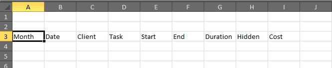
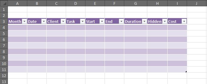
In the “Main/Data” sheet type the column headings shown below in row 3 – don’t worry about any formatting just yet…
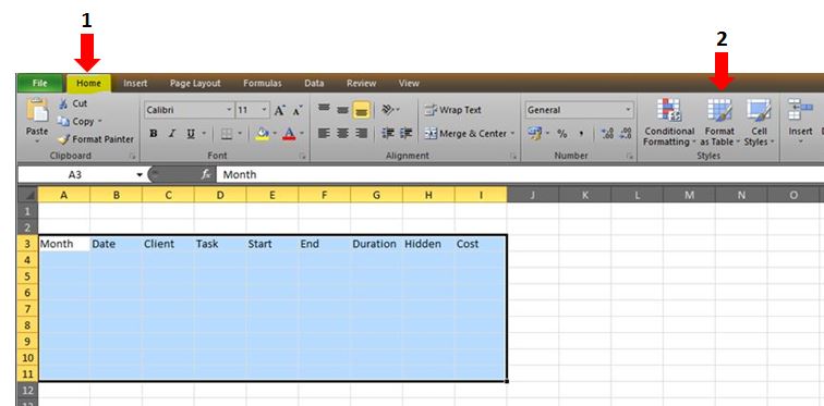
Next we need to format these headings as a table. Highlight the headings you’ve just typed down to about row 11 (so from cell A3 to cell I11). In the Home tab on the ribbon, go to the Styles group & click Format as Table…
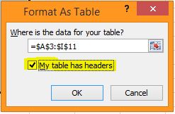
Choose a design you like from the drop down selection, and tick the box My table has headers…
Your table will now appear in the colour/design you chose, the column headers in the table will be in bold and the filter has automatically been added to each column…
Next we need to create the lists which will be used for data validation. We’ll be formatting the columns for Client and Task so that we select the options from a drop down arrow – this will save on typing!
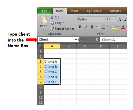
Go to the “Lists” sheet and start typing in the relevant information. The first list in column A will be your Client name. Once you’ve added the names you require highlight them all and type “Client” into the Name Box which is located between the ribbon and column header A / B, and press return…
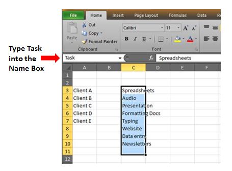
Do the same for the tasks list – type your tasks into column C, highlight the list, type “Task” into the Name Box and press return…
So, we now have everything all ready for the formulas to be entered into the main table which we’ll cover in the next tutorial. If you have any questions regarding any of the above steps, please comment below 🙂