
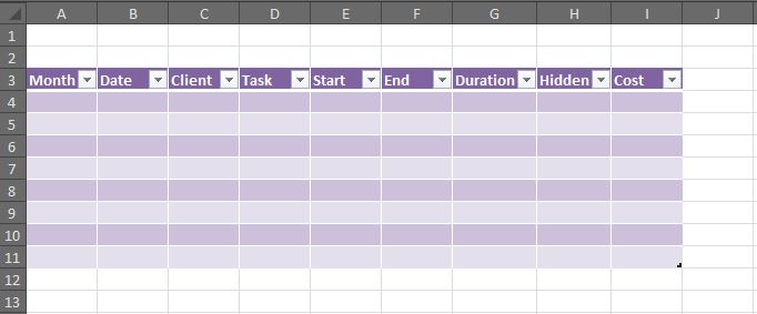
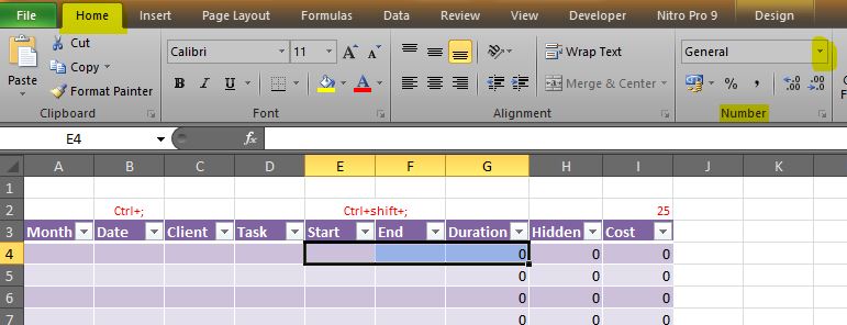
Continuing on from Part 1 in the series of creating a timesheet in Excel, this post will show you a breakdown of the formulas used to calculate everything that’s needed in the timesheet. Below is the spreadsheet (in “Main” sheet) we created in part 1 (click on the image to enlarge)…
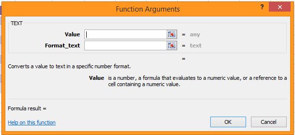
Column A: Month – this column will contain the actual month written in full taken from the Date column. Rather than manually typing out the month each time, we can add a formula to this column instead. The formula used is the “Text” function, this converts a value into a specific format…
So we click into cell A4 and type the following formula:
=TEXT(B4,”mmmm”)
Cell B4 is where the value is located that we want to format – so this is the Date column. TIP: instead of typing B4 you can just click onto that cell & it will input the actual table header “Date” into the formula instead.
“mmmm” is the date format we want to use – this displays the month in full; if we only wanted to see 3 letters of the month then we would type “mmm”. You’ll see it automatically has January as the answer – this is default as there is no date included in column B as of yet. In order to get rid of this, we can add the IF function to the formula…
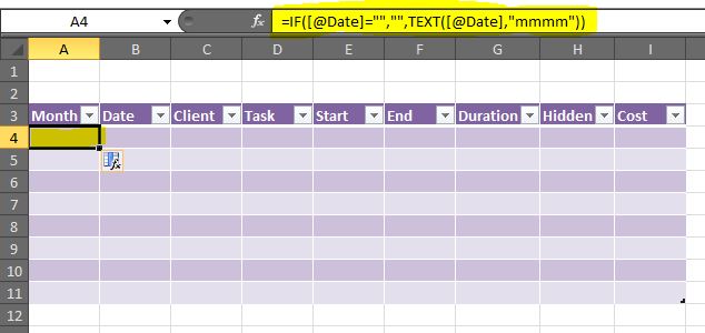
Basically we want to say that IF cell B4 is blank then leave cell A4 blank, otherwise put in the text formula. This is written as follows in cell A4:
=IF(B4=””,””,TEXT(B4,”mmmm”))
Press return and you’ll see that A4 is now blank – there is still a formula in there as seen in the formula bar…
Try putting a date in cell B4 & you’ll see cell A4 change to that month.
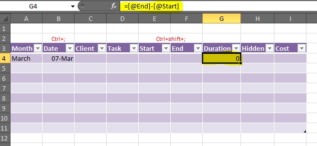
In columns B, E and F we can use a keyboard shortcut to save time…
Column B: Date – Type Ctrl+; to automatically insert today’s date.
Column E & F: Start & End – Type Ctrl+shift+; to insert the current time.
Note – We’ve missed out columns C and D (Client and Task) as these will be formatted for data validation which we’ll cover in the next tutorial.
Column G: Duration – this column has a simple formula of the End time minus the Start time. Click into cell G4 and type the following formula:
=F4-E4
TIP: again you can click onto the cells instead of typing F4 and E4 & it will input the actual table headers “End” and “Start” into the formula instead.
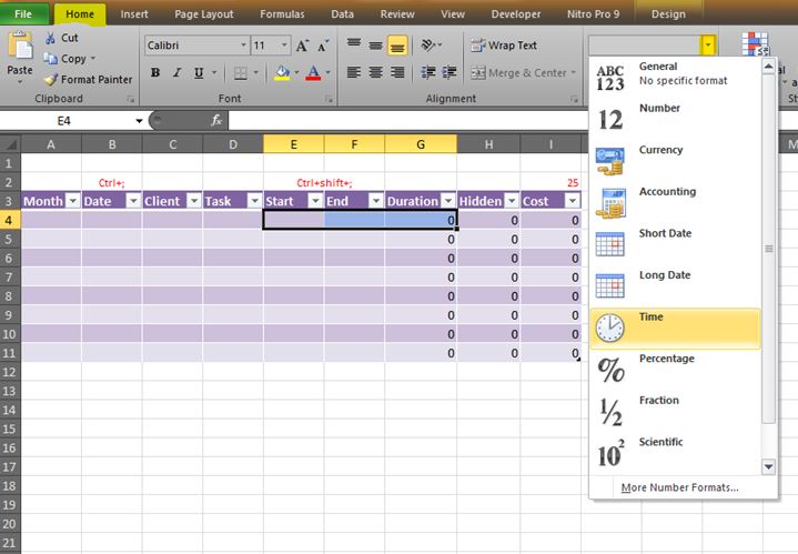
If you type in a start and end time you’ll notice that the duration time isn’t formatted correctly. To quickly change this, highlight cells E4 to G4 and go to the Number section in the Home tab of the ribbon. Click on the drop down arrow next to General, and select the Time format…
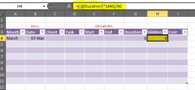
Column H: Hidden – this column will be hidden once the table is complete. It will contain the formula to work out the decimal value of the duration (in order to make it easier to calculate the cost). In cell H4 type the following formula:
=(G4*1440)/60
This is the duration multiplied by 1440 (the number of minutes in a day) divided by 60 to get the hourly decimal value…
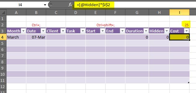
Column I: Cost – this column works out what the charge would be for that particular time. In this example I’m using my hourly rate of €25. I insert 25 into cell I2 (above the actual table) which will be used in the formula. In cell I4 type the following formula:
=H4*I2
This is multiplying the decimal value by the hourly rate. However if we copy this formula down the column, the cell containing the hourly rate (I2) will also move down one row each time, so we need to “fix” this cell as an absolute reference, so that particular cell remains constant when the formula is copied down. To do this put the dollar sign before the I and 2 as follows:
=H4*$I$2
And that’s it! They’re the formulas needed to calculate the basics in the timesheet.
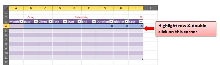
We can now copy these down the rest of the table. Highlight row 4 of the table and go to the bottom right corner of the highlighted area. You’ll see that your cursor changes to a single black cross. Double click and it will copy everything down to the bottom of the table…
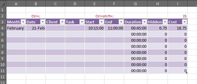
So the table should look like this (I’ve filled in the first row as an example)…
The next tutorial will show how to add the data validation cells & also a general tidy up / formatting to make the table more visually pleasing 🙂