In this tutorial we’ll be formatting the table in Excel ready for data validation and also doing a general tidy up. Last time we made sure our timesheet had all the relevant formulas included so the basics are now ready 🙂

The 2 columns which we’ll format first are C (Client) and D (Task). If you look back to Part 1 in this series you’ll remember that we created 2 lists named Client and Task in another sheet (which we named Lists).

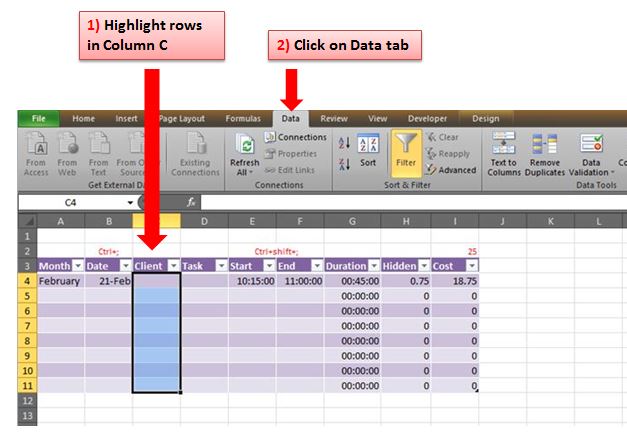
To start, click in the table and highlight the rows in column C (Client), then click the Data tab on the ribbon…

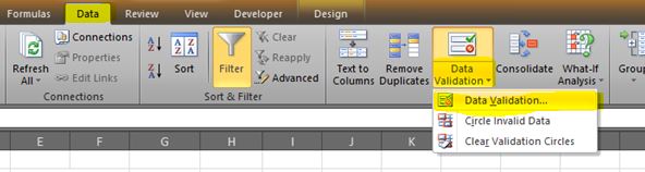
Click on the drop down arrow next to Data Validation, then select Data Validation…

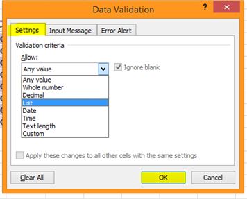
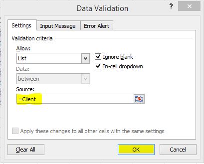
In the Settings tab click on the drop down arrow under Allow: this sets the value which is allowed within the highlighted cells in the table. We want to choose List…

We then need to state the Source i.e. where the list is located. There are 2 ways to do this:-

1. Click on the icon on the right hand side of the Source box, then click into the Lists sheet, highlight the Client list then click back on the icon and press OK…

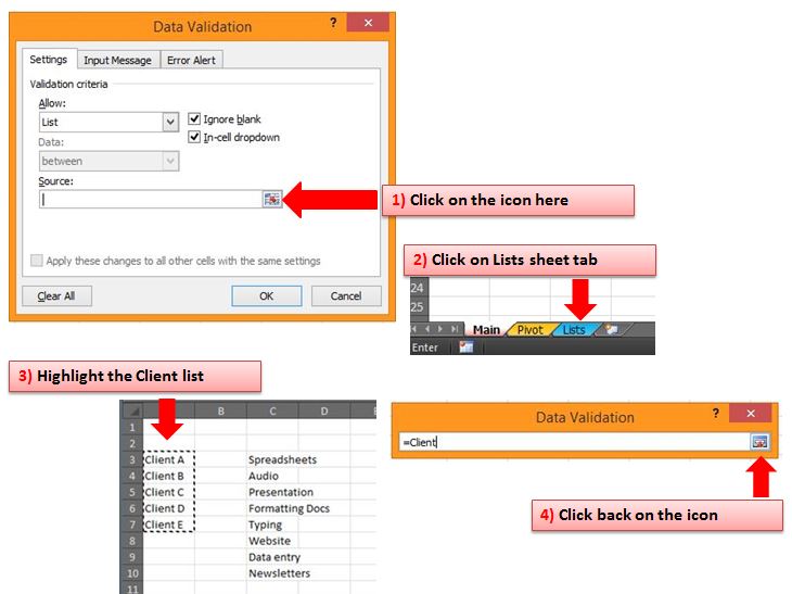
 2. If we know the name of the List which we created in Part 1, then we can just type in =Client and press OK…

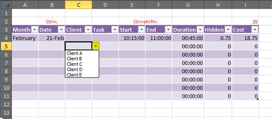
Either of the methods above work so it’s up to you which you prefer to use.  If we now click back into any cell under the Client heading in the table, you’ll see a drop down arrow appear. Click on the arrow and the Client list will now show…

We now need to do the same with the Task column, so repeat the steps above…

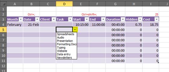
1) Highlight the cells in column D under Task… -> 2) Click on the Data tab on the ribbon, click on the drop down arrow next to Data Validation, and select Data Validation… -> 3) Click on the drop down arrow under Allow and choose List… -> 4) Type “=Task” into the Source box… -> 5) Click OK.

We now have a list of tasks available to choose from in the drop down arrow when we click on any cell under the Task heading in the table…

Our table is now ready to begin the tidy up. All of the following is based on my own personal preference, so if you don’t want certain columns to be centred or if you want the currency to be different, then you can choose how you want to format it.

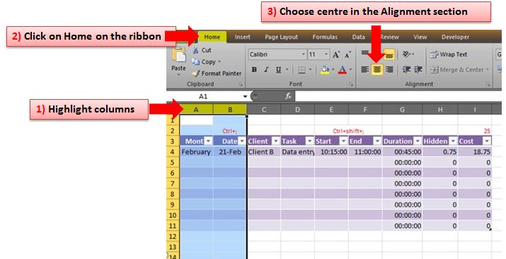
Firstly I would start with the alignment of text so I would begin with centering the first 2 columns – highlight Columns A & B and choose centre in the Alignment section of the Home tab on the ribbon…

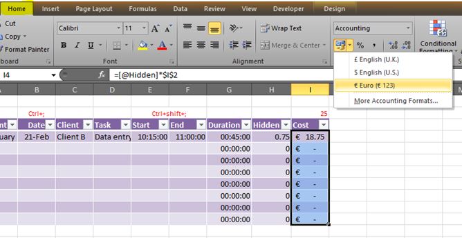
Next I would format the Cost column to show the Euro currency. Highlight the column under Cost and click on the icon for Accounting Number Format in the Number section of the Home tab on the ribbon, then choose Euro…

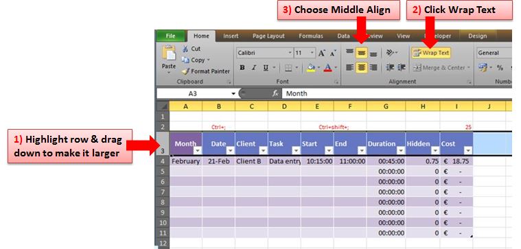
Next I would make the table headers slightly deeper and wrap the text centrally.  Highlight row 3 and drag the height of the row down a little, click on Wrap Text in the Alignment section of the Home tab on the ribbon, and choose Middle Align…

That would probably be sufficient for the time being. We can now hide column H (Hidden) – right click on the column and select Hide. TIP: Click anywhere in the column & use the keyboard shortcut Ctrl+0 to hide the column.

And that’s it – we can now start populating the timesheet as & when needed. Use the Tab key to move from one cell to the next along the rows and when you reach the end of the table press tab again and it will automatically create a new row underneath containing all the formulas and formatting.

TIP: If some of the text doesn’t fit in the columns, double click on the vertical line to the right of the column header (e.g. the line separating the column header D & E) and it will automatically resize to fit the widest cell containing text.

My next tutorial will show what to do with the data now that you have it & will look at pivot tables and charts. If you have any questions on any of the above, please feel free to comment below 🙂