A few weeks ago I asked followers of my Facebook page if they wanted me to cover a specific topic in a tutorial, the majority of the replies I received were for pivot tables. It seems a lot of people want to use them but are just not sure where to begin, so in the words of Aladdin’s genie “your wish is my command”! 🙂

Firstly, for those of you who don’t know what a pivot table is, it’s a fantastic tool in Excel that sorts and summarises data, and then inputs it into another table which is a bit more user friendly, more readable.  For example, if you have data that shows details of every customer that has bought your product over the last 5 years, by using a pivot table you can find out which product is most popular, which town/county/country most of your customers came from, and whether your customers were male or female etc, depending on the data you have available.

Below is a short tutorial on how to set up a very simple pivot table in Excel 2007.

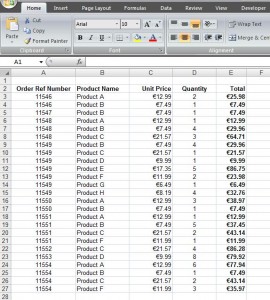
In Sheet 1 is a list of data that we’ll use for the pivot table, it basically just lists a reference number, product name, unit price, quantity and a total…

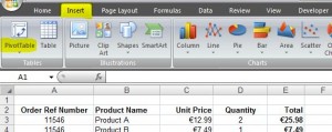
Go to the Insert tab on the Ribbon and select PivotTable…

This opens up a new dialogue box where you select the range of data that you want to use for the pivot table (in this example it has automatically highlighted the range A2:E27), and where you want the pivot table to appear either in a new worksheet or the existing one.  For this example we’ll choose existing worksheet, and we’ll click on a blank cell of where the pivot table is to go e.g. cell G2.  Click OK…

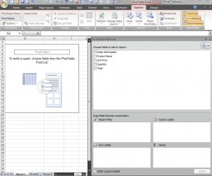
You’ll notice the Pivot Table Field List opens up and tools become available for the pivot table…

Choose the fields that you want to appear in the pivot table by dragging them into the relevant sections (Report, Row, Column, and Values).  For this example, we’ll choose the Order Ref Number field to the Row section and the Total to the Values section…

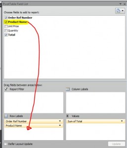
If we change our mind and decide that we want to see the product name instead of the reference number, all we do is click on Product Name and drag it down to the Row section like we did with the others…

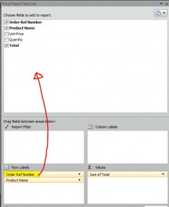
Then, to remove the Order Ref Number, you can either click and drag the field back up to the top…

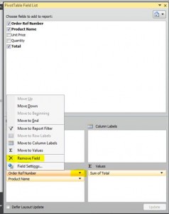
…or click on the drop down arrow next to Order ref Number and choose Remove Field…

…or just un-tick the Order Ref Number option…

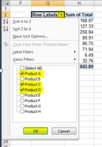
Whichever way you choose, the field will disappear from the pivot table leaving you with just the Product Name and Total.  The pivot table automatically applies a filter so you can choose which data you want to see, for example you may only want to see Product Names A, C and D, just click on the drop down arrow next to the title and tick the boxes of ones you want to see…

Obviously this tutorial is just showing you the basics, a lot of creating a pivot table is trial & error and it’s just a matter of working out the best way of organising the data you want to see.  There are other options within it to allow different formats of fields, different views etc.  Pivot tables are so flexible so once you have the basic one set up, just have a play around with the data.  The next tutorial will show you how to format your table and what to do if the original data changes.

I hope you find this useful, but if you have any questions about this tutorial, please leave them in the comment section below 🙂